強化学習モデル: ベイズ推定(2)
認知モデリングの推奨実践法
Busemeyer & Diederich(2010), Heathcote (2014), Palminteri et al.(2017)を参考にまとめると,以下のような感じになります。
- A 認知課題と認知モデルを準備
- B 人工データ生成とパラメータリカバリーを確認(モデルや課題の修正)
- C データ収集と行動データを確認
- D パラメータ推定
- E 相対モデル比較
- F モデル・シミュレーションと選択的影響テスト
「強化学習モデル: 最尤推定」と「強化学習モデル: ベイズ推定(1)」では,ABCDとすすめてきました。今回は,今回は,EとFについて説明します(相対モデル比較に関連づけてモデル・リカバリーの説明もします)。
使用するRパッケージ
適宜必要なパッケージをインストールしてください(「強化学習モデル: ベイズ推定(1)」と同じです)。
rm(list = ls())
library(tidyverse)
library(cmdstanr)
library(rstan)
library(posterior)
library(bridgesampling)
「強化学習モデル: ベイズ推定(1)」と同じく,人工データを生成するために,実験状況の入ったsim_dataの準備とq_learning_sim関数を準備をします。
sim_data <- tibble(trial = 1:80,
                   prob_s1 = rep(c(0.2, 0.8), each = 40),
                   prob_s2 = rep(c(0.8, 0.2), each = 40),
                   reward_s1 = ifelse(runif(80) < prob_s1, 1, 0),
                   reward_s2 = ifelse(runif(80) < prob_s2, 1, 0))

q_learning_sim <- function(alpha, beta,data) {
  #変数の準備
  value_s1 <- 0          # s1の価値(初期値は0)
  value_s2 <- 0          # s2の価値(初期値は0)
  current_choice <- NULL     # ある時点の選択(1=s1,0=s2)
  choice_prob_s1 <- NULL  # s1の選択確率
  reward <- NULL                 # 報酬
  # Qlearningモデル
  for (i in 1:nrow(data)){
    # s1を選ぶ確率を計算し,一様分布から発生させた乱数が行動選択確率よりも小さい時に1(s1),大きい時に0(s2)
    choice_prob_s1[i] <- exp(beta*value_s1[i])/(exp(beta*value_s1[i])+exp(beta*value_s2[i]))
    current_choice[i] <- as.integer(runif(1,min=0,max=1) <= choice_prob_s1[i])
    #FBを報酬(r)として、価値の更新を行う。
    if (current_choice[i] == 1){
        reward[i] <- data$reward_s1[i]
        #予測誤差の計算
        prediction_error <-  reward[i] - value_s1[i]
        #予測誤差を使ってs1の価値を更新する
        value_s1[i+1] <- value_s1[i]+alpha*prediction_error
        #s2は更新なし
        value_s2[i+1] <- value_s2[i]
    }else{
        reward[i] <- data$reward_s2[i]
        #予測誤差の計算
        prediction_error <- reward[i] - value_s2[i]
        #予測誤差を使ってs2の価値を更新する
        value_s2[i+1] <- value_s2[i]+alpha*prediction_error
        #s1は更新なし
        value_s1[i+1] <- value_s1[i]
    }
  }
  result <- data.frame(trial = data$trial,
              value_s1 = value_s1[1:nrow(data)],
              value_s2 = value_s2[1:nrow(data)],
              prob_s1 = choice_prob_s1,
              choice = current_choice,
              reward = reward)
  return(result)
}

# データの準備
setwd("data")
file_names <- list.files()
setwd("..")
# 確認用の図を入れる場所を確保
plot_check <- NULL
# データを入れる場所を確保
data_long <- NULL
for (i in 1:length(file_names)) {
  # file_namesのi番目のデータを読み込んで,上記の処理をして,tmp_dataに格納
  tmp_data <- read_csv(paste("data",file_names[i], sep = "/")) %>%
    filter(trial_type == "html-button-response") %>%
    mutate(id = rep(i,80),
           trial = 1:80,
           s1_prob = rep(c(0.2,0.8),each = 40),
           reward = ifelse(button_pressed == 0, reward_s1, reward_s2)) %>%
    select(id, trial,choice=button_pressed, rt, reward, s1_prob,reward_s1, reward_s2)
  # データの保存
  data_long <- rbind(data_long, tmp_data)
}
E 相対モデル比較
ここでは,sub02を対象にして,モデル比較をしてみたいと思います。モデル比較する場合には,以下の2種類があります。今回は,予測をしたいという話ではないので,WBICを使用します。
予測の良さに基づくモデル選択法:KL距離をベースにしたものであり,予測をする上で悪いものを避けるという保守的なモデル選択ができる。例えば,AIC, DIC,WAICなどがあります。
ベイズ的なモデル選択法(モデルと事前分布からみてどのくらいデータが意外か。この意外性が小さいほど良いモデルと考えられる):BIC, WBIC, ベイズファクター,自由エネルギー
WBICの計算をする場合は,stanコードの対数尤度の計算の部分で対数尤度に(1/log(データ数)) を掛ける必要があります。さらに,generated quantitiesブロックで対数尤度を計算します。それぞれは,以下になります。
- q_learning_WBIC.stan
data {
  int<lower=1> trial;
  array[trial] int<lower=1,upper=2> choice; // 1 or 2
  array[trial] int<lower=0,upper=1> reward; // 0 or 1
}
parameters {
  real<lower=0.0,upper=1.0> alpha; //学習率
  real<lower=0.0> beta;            //逆温度
}
model {
  //学習率と逆温度の事前分布の指定はしていないので,parametersで指定した範囲の無情報事前分布が使われる
  matrix[trial,2] Q;
  Q[1, 1] = 0;
  Q[1, 2] = 0;

  for ( t in 1:trial) {
    // 対数尤度を足す
    target += (1/log(trial))*log(exp(beta*Q[t,choice[t]])/(exp(beta*Q[t,choice[t]])+exp(beta*Q[t,3-choice[t]])));

    if (t < trial) {
      // 選択された選択肢のQ値の更新
      Q[t+1,choice[t]] = Q[t, choice[t]] + alpha * (reward[t] - Q[t, choice[t]]);
      // 選択されなかった選択肢は更新しない
      Q[t+1, 3- choice[t]] = Q[t, 3- choice[t]];
    }
  }
}
generated quantities {
  vector[trial] log_lik;
  {
    matrix[trial, 2] Q;
    Q[1, 1] = 0;
    Q[1, 2] = 0;
    for ( t in 1:trial ) {
       log_lik[t] =  log(exp(beta*Q[t,choice[t]])/(exp(beta*Q[t,choice[t]])+exp(beta*Q[t,3-choice[t]])));
      if (t < trial) {
        // 選択された選択肢のQ値の更新
        Q[t+1,choice[t]] = Q[t, choice[t]] + alpha * (reward[t] - Q[t, choice[t]]);
        // 選択されなかった選択肢は更新しない
        Q[t+1, 3- choice[t]] = Q[t, 3- choice[t]];
      }
    }
  }
}
- q_learning_prior_WBIC.stan
data {
  int<lower=1> trial;
  array[trial] int<lower=1,upper=2> choice; // 1 or 2
  array[trial] int<lower=0,upper=1> reward; // 0 or 1
}
parameters {
  real<lower=0.0,upper=1.0> alpha; //学習率
  real<lower=0.0> beta;            //逆温度
}
model {
  matrix[trial,2] Q;
  Q[1, 1] = 0;
  Q[1, 2] = 0;

  //学習率の事前分布にベータ分布,逆温度の事前分布にガンマ分布
  alpha ~ beta(1.2, 1.2);
  beta ~ gamma(4.82, 0.88);

  for ( t in 1:trial) {
    // 対数尤度を足す
    target += (1/log(trial))*log(exp(beta*Q[t,choice[t]])/(exp(beta*Q[t,choice[t]])+exp(beta*Q[t,3-choice[t]])));

    if (t < trial) {
      // 選択された選択肢のQ値の更新
      Q[t+1,choice[t]] = Q[t, choice[t]] + alpha * (reward[t] - Q[t, choice[t]]);
      // 選択されなかった選択肢は更新しない
      Q[t+1, 3- choice[t]] = Q[t, 3- choice[t]];
    }
  }
}
generated quantities {
  vector[trial] log_lik;
  {
    matrix[trial, 2] Q;
    Q[1, 1] = 0;
    Q[1, 2] = 0;
    for ( t in 1:trial ) {
       log_lik[t] =  log(exp(beta*Q[t,choice[t]])/(exp(beta*Q[t,choice[t]])+exp(beta*Q[t,3-choice[t]])));
      if (t < trial) {
        // 選択された選択肢のQ値の更新
        Q[t+1,choice[t]] = Q[t, choice[t]] + alpha * (reward[t] - Q[t, choice[t]]);
        // 選択されなかった選択肢は更新しない
        Q[t+1, 3- choice[t]] = Q[t, 3- choice[t]];
      }
    }
  }
}
WBICによるモデル比較
推定してモデル比較してみましょう。まずは,モデルをコンパイルします。
q_learning_WBIC <- cmdstan_model('q_learning_WBIC.stan')
q_learning_prior_WBIC <- cmdstan_model('q_learning_prior_WBIC.stan')
それでは,sub02で推定をしてみましょう!
data_individual <- data_long %>%
  filter(id == 2)

q_learning_WBIC_mcmc <- q_learning_WBIC$sample(
        data = list(trial = nrow(data_individual),
                   reward = data_individual$reward,
                   choice = data_individual$choice + 1),
        seed = 123,
        chains = 4,
        iter_warmup = 500,
        iter_sampling = 3000,
        parallel_chains = 4)

q_learning_prior_WBIC_mcmc <- q_learning_prior_WBIC$sample(
        data = list(trial = nrow(data_individual),
                   reward = data_individual$reward,
                   choice = data_individual$choice + 1),
        seed = 123,
        chains = 4,
        iter_warmup = 500,
        iter_sampling = 3000,
        parallel_chains = 4)

q_learning_WBIC_sample <- rstan::read_stan_csv(q_learning_WBIC_mcmc$output_files())
q_learning_prior_WBIC_sample <- rstan::read_stan_csv(q_learning_prior_WBIC_mcmc$output_files())
sub02について,WBICを確認したところ,情報事前分布の方がWBICが低くなりました。なお,sub01においては,無情報事前分布の方がWBICは低くなっています。ただし,sub01もsub02も無情報事前分布では,十分な収束ができておらず,そもそもモデル比較の前の問題があります。
WBIC_non <- -mean(rowSums(rstan::extract(q_learning_WBIC_sample)$log_lik))
WBIC_prior <- -mean(rowSums(rstan::extract(q_learning_prior_WBIC_sample)$log_lik))
paste("無情報事前分布のWBICは",WBIC_non)
## [1] "無情報事前分布のWBICは 51.712855984715"paste("有情報事前分布のWBICは",WBIC_prior)## [1] "有情報事前分布のWBICは 49.5467001469408"モデルリカバリー(Model Recovery)
これまでパラメータリカバリーをパラメータ推定のチェックに用いてきました。特定のモデルのパラメータ推定の精度を調べる上では,パラメータリカバリーが使えます。ただし,そもそもデータ生成に用いたれたモデルがモデル選択でちゃんと選ばれるのかについては,検討ができていません。生成モデルはあくまで研究者が仮定したものであって,複数の生成モデルが存在すると考えられるので,データからちゃんとモデルが選択できることが重要です。
パラメータ推定後の相対モデル比較において,データ生成過程で用いられた生成モデルがちゃんと選ばれるか確認するモデルリカバリーという考えがあります(Wilson & Collins, 2019)。例えば,特定の生成モデルAから生成されたシミュレーションデータに対して,複数の生成モデルA ,B,Cを用いてパラメータ推定してモデル比較した場合,BやCよりもAが選ばれる必要があります。これを検討するのがモデルリカバリーです。モデルリカバリーでは,全ての生成モデルから異なる値のパラメータを用いてシミュレーションデータを生成し,それらに対して,全ての生成モデルを用いてパラメータ推定を行うことを全ての組み合わせで行います。モデルリカバリーによって,検討しているモデルが研究目的から妥当か,追加すべきモデルはないか,パラメータ推定で識別不可能なモデルはないかを検討することができます。
モデルリカバリーで用いるモデル
あまり複雑にしないために,これまで用いてきたモデルとそのモデルを一部改変したモデルを考えます。
- 上記で検討した情報事前分布をおいた強化学習モデル(Model 1)
- 上記からβを除外した強化学習モデル(Model 2, β=1に仮定したモデルともいえます)
αとβを仮定したモデル(Model 1)から生成されたデータのモデルリカバリー
まずは,これまでと同様なαもβも存在する強化学習モデル(Model 1)でデータを生成します。それに対して,それと一致したモデル(Model 1, 上記のq_learning_prior_WBIC.stan)と一致しないモデル(Model 2, 以下のq_learning_prior_non_beta_WBIC.stan)を使って推定することで,モデルリカバリーをします。
q_learning_prior_non_beta_WBIC.stanは,以下のようなコードになります。簡単にいうと,q_learning_weak_info_single_WBIC.stanからbetaを抜いただけです。
data {
  int<lower=1> trial;
  array[trial] int<lower=1,upper=2> choice; // 1 or 2
  array[trial] int<lower=0,upper=1> reward; // 0 or 1
}

parameters {
  real<lower=0.0,upper=1.0> alpha; //学習率
}

model {
  matrix[trial,2] Q;
  Q[1, 1] = 0;
  Q[1, 2] = 0;
  //学習率の事前分布にベータ分布
  alpha ~ beta(1.2, 1.2);
  for ( t in 1:trial) {
    // 対数尤度を足す
    target += (1/log(trial))*log(exp(Q[t,choice[t]])/(exp(Q[t,choice[t]])+exp(Q[t,3-choice[t]])));

    if (t < trial) {
      // 選択された選択肢のQ値の更新
      Q[t+1,choice[t]] = Q[t, choice[t]] + alpha * (reward[t] - Q[t, choice[t]]);
      // 選択されなかった選択肢は更新しない
      Q[t+1, 3- choice[t]] = Q[t, 3- choice[t]];
    }
  }
}

generated quantities {
  vector[trial] log_lik;
  {
    matrix[trial, 2] Q;
    Q[1, 1] = 0;
    Q[1, 2] = 0;
    for ( t in 1:trial ) {
       log_lik[t] =  log(exp(Q[t,choice[t]])/(exp(Q[t,choice[t]])+exp(Q[t,3-choice[t]])));
      if (t < trial) {
        // 選択された選択肢のQ値の更新
        Q[t+1,choice[t]] = Q[t, choice[t]] + alpha * (reward[t] - Q[t, choice[t]]);
        // 選択されなかった選択肢は更新しない
        Q[t+1, 3- choice[t]] = Q[t, 3- choice[t]];
      }
    }
  }
}
まずは,q_learning_prior_non_beta_WBIC.stanをコンパイルします。
q_learning_prior_non_beta_WBIC <- cmdstan_model('q_learning_prior_non_beta_WBIC.stan')さて,以下のコードを走らせて,αとβを仮定したモデル(Model 1)で生成されたデータをαとβを仮定するモデル(Model 1)とαだけを仮定するモデル(Model 2)でフィッティングした時に,モデルが選択される確率を計算します。以下では,100回シミュテーションデータを生成して,MCMCで推定をするのでかなり時間がかかると思います(メモリもかなり使うと予想されます)。
better_model1 <- 0
n_simulation <- 100
for (i in 1:n_simulation) {
  alpha_set <- rbeta(1, 1.2, 1.2)
  beta_set <- rgamma(1, 4.82, 0.88)
  #データ生成
  data_2 <- q_learning_sim(alpha = alpha_set, beta = beta_set, sim_data)
  print(paste("進捗状況:",i,"/",n_simulation))
  #パラメータ推定(推定がミスった時用にtryCatch関数を準備)
  tryCatch({
    with_beta_WBIC <- q_learning_prior_WBIC$sample(
      data = list(trial = nrow(data_2),
                   reward = data_2$reward,
                   choice = data_2$choice + 1),
      seed = 123,
      chains = 4,
      iter_warmup = 500,
      iter_sampling = 3000,
      parallel_chains = 4)

    non_beta_WBIC <- q_learning_prior_non_beta_WBIC$sample(
      data = list(trial = nrow(data_2),
                   reward = data_2$reward,
                   choice = data_2$choice + 1),
      seed = 123,
      chains = 4,
      iter_warmup = 500,
      iter_sampling = 3000,
      parallel_chains = 4)

    with_beta_WBIC_sample <- rstan::read_stan_csv(with_beta_WBIC$output_files())
    WBIC_with_beta <- -mean(rowSums(rstan::extract(with_beta_WBIC_sample)$log_lik))
    non_beta_WBIC_sample <- rstan::read_stan_csv(non_beta_WBIC$output_files())
    WBIC_no_beta <- -mean(rowSums(rstan::extract(non_beta_WBIC_sample)$log_lik))
    better_model1 <- better_model1 + ifelse(WBIC_with_beta < WBIC_no_beta, 1, 0)
  },error = function(e) {message(e)})
}

fit_model1_sim_model1 <- better_model1/n_simulation
fit_model2_sim_model1 <- (n_simulation - better_model1) / n_simulation
αのみを仮定したモデル(Model 2)から生成されたデータのモデルリカバリー
次は,αのみを仮定したモデル(Model 2, βは仮定しない,つまり,βを1に固定するモデル)で生成されたデータをαとβを仮定するモデル(Model 1)とαだけを仮定するモデル(Model 2)でフィッティングした時に,モデルが選択される確率を計算します。以下では,100回シミュテーションデータを生成して,MCMCで推定をするのでかなり時間がかかると思います(メモリもかなり使うと予想されます)。
better_model1 <- 0
n_simulation <- 100
beta_set <- 1
for (i in 1:n_simulation) {
    alpha_set = runif(1,0, 1)
    #データ生成
    data_2 <- q_learning_sim(alpha = alpha_set, beta = beta_set, sim_data)
    print(paste("進捗状況:",i,"/",n_simulation))
    #パラメータ推定(推定がミスった時用にtryCatch関数を準備)
    tryCatch({
      with_beta_WBIC <- q_learning_prior_WBIC$sample(
        data = list(trial = nrow(data_2),
                   reward = data_2$reward,
                   choice = data_2$choice + 1),
        seed = 123,
        chains = 4,
        iter_warmup = 500,
        iter_sampling = 3000,
        parallel_chains = 4)

      non_beta_WBIC <- q_learning_prior_non_beta_WBIC$sample(
        data = list(trial = nrow(data_2),
                   reward = data_2$reward,
                   choice = data_2$choice + 1),
        seed = 123,
        chains = 4,
        iter_warmup = 500,
        iter_sampling = 3000,
        parallel_chains = 4)

    with_beta_WBIC_sample <- rstan::read_stan_csv(with_beta_WBIC$output_files())
    WBIC_with_beta <- -mean(rowSums(rstan::extract(with_beta_WBIC_sample)$log_lik))
    non_beta_WBIC_sample <- rstan::read_stan_csv(non_beta_WBIC$output_files())
    WBIC_no_beta <- -mean(rowSums(rstan::extract(non_beta_WBIC_sample)$log_lik))
    better_model1 <- better_model1 + ifelse(WBIC_with_beta < WBIC_no_beta, 1, 0)
  },error = function(e) {message(e)})
}

fit_model1_sim_model2 <- better_model1 / n_simulation
fit_model2_sim_model2 <- (n_simulation - better_model1) / n_simulation
ヒートマップ形式で図示します。
- alphaとbetaの両方があるモデル(Model 1)で生成したデータのパラメータ推定で,alphaとbetaの両方があるモデル(Model 1)の方が高い確率で選択されています。
- alphaだけのモデル(Model2)で生成したデータのパタメータ推定で,alphaだけのモデル(Model2)の方が高い確率で選択されています。
偶然,設定したβが1付近になってモデル識別が難しくなるケースがあったりするかもしれません。なお,今回は100回だけにしていますが,繰り返し回数を増やしたほうが良いかもしれません。
simulated_model <- factor(c("Model 1","Model 1","Model 2","Model 2"), levels = c("Model 2","Model 1"))
fit_model <- factor(c("Model 1","Model 2","Model 1","Model 2"), levels = c("Model 1","Model 2"))
Probability <- c(fit_model1_sim_model1, fit_model2_sim_model1, fit_model1_sim_model2, fit_model2_sim_model2)
model_recovery <- tibble(simulated_model, fit_model, Probability)

ggplot(model_recovery, aes(x = fit_model, y = simulated_model, fill = Probability)) +
  geom_tile() +
  scale_fill_gradient(low = "white", high = "red") +
  geom_text(aes(label = round(Probability, digits = 2)), color = "black") +
  xlab("Fit Model") +
  ylab("Simulated Model")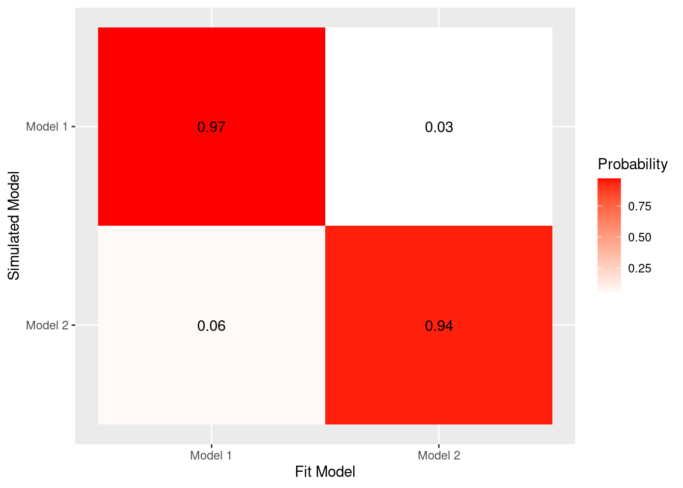
F モデル・シミュレーションと選択的影響テスト
モデル・シミュレーションでは,「強化学習モデル: 最尤推定」で行ったような人工データ生成を最もフィットの良かった推定値を用いて行います。複数のモデルの中で最もデータ適合が良いモデルであったとしても,それは相対的に良いモデルになります。私達が想定したモデルはどれも悪いモデルだった場合は,相対的には良いモデルを選ぶことはできても,それが絶対的には悪いモデルある可能性があります。そこで,情報量規準などで最も良いとされたモデルの推定値を用いて,人工データ生成を行って,その生成されたデータが現実のデータに近いものかを評価します。モデルシミュレーションについては,Palminteri, Wyart, & Koechlin(2017)が詳しいです。
選択的影響テストとは,実験的操作を用いて,認知モデルの妥当性を検討する方法です(Heathcote et al., 2015)。選択的影響テストでは,認知モデルの特定のパラメータに影響すると考えられる実験的な操作をして,実際にパラメータに変化が生じるのかを検討します。この予想された変化をもって,パラメータとモデルの妥当性を示すことができます。例えば,反応時間に関する Drift-Diffusion Modelの妥当性検討では,色識別課題の条件を操作することで,操作に対応したパラメータの変化を確認していたりします(Voss, Rothermund, and Voss , 2004)。
引用・参考文献
- Busemeyer, J. R., & Diederich, A. (2010). Cognitive Modeling. SAGE.
- Heathcote, A., Brown, S. D., & Wagenmakers, E.-J. (2015). An Introduction to Good Practices in Cognitive Modeling. In B. U. Forstmann & E.-J. Wagenmakers (Eds.), An Introduction to Model-Based Cognitive Neuroscience (pp. 25–48). Springer New York.
- Palminteri, S., Wyart, V., & Koechlin, E. (2017). The Importance of Falsification in Computational Cognitive Modeling. Trends in Cognitive Sciences, 21(6), 425–433.
- Voss, A., Rothermund, K., & Voss, J. (2004). Interpreting the parameters of the diffusion model: an empirical validation. Memory & Cognition, 32(7), 1206–1220.
- Wilson, R. C., & Collins, A. G. (2019). Ten simple rules for the computational modeling of behavioral data. eLife, 8. https://doi.org/10.7554/eLife.49547